This is the second part of a five part series. Check out Part 1, Part 3, Part 4, Part 5 here. You can view the series both at Hockey-Graphs.com and APHockey.net.

In Part 1, I looked at some of the theory behind Pythagorean Expectations and their origin in baseball. You can find the original formula copied below.

WPct = W/(W+L) = Runs^2/(Runs^2 + Runs Against^2)

The idea behind the formula is that it is a skill to be able to score runs and to be able to prevent them. What isn’t a skill, however — according to the theory — is when one scores or allows those runs. Teams over the course of weeks or months may appear to be able to score runs when they’re most necessary, to squeak out one-run wins, but as much as it looks like a pattern, it is most often simple variance. If you don’t fully buy into that idea, or you don’t really understand what I mean by variance, read this and then come back. Everything should be a lot clearer.

When applying Pythagorean Expectations to hockey, there are a couple of factors that complicate the matter. First of all, the goal/run scoring environment is very different. Hockey is a much lower scoring sport. That means that a team is more likely to win, say, 10 one-goal games in a row than in baseball. The lower the total goals, the closer the average scores, the more variance involved. Second, not all games are worth the same number of points. In baseball, you either win or lose, so you use run differential to figure out a winning percentage. But winning percentage doesn’t really work as a statistic in hockey since you can lose in overtime and get essentially half a win, while your opponent gets a full win.

I’m far from the first one to look at Pythagorean Expectations in hockey. Alan Ryder wrote this fantastic piece back in 2004 examining different ways of predicting a team’s record, and brainstormed on how to adapt for the differences mentioned above. A number of others have picked up on the idea since, but now that shootouts have entered the picture and goal scoring has once again dropped, it’s important to revise and re-examine the issue. And as I mentioned, this series is more about the ability to exceed one’s expectation rather than the exact correct method of determining it in the first place.

But allow me to dive into the five variations in method I looked at to determine the ideal exponent in James’ formula applied to hockey, while accounting for the idea of ties and three-point games in the sport.

1. Log Ratios

One of the most common ways to find the ideal exponent for the Pythagorean formula in baseball involves log ratios, so we’ll start there. First of all, we have to use some algebra to alter the formula to our liking. Instead of using wins and losses, we use points and (potential points – points), or points lost essentially. Every team’s potential point total to start a season is 164. So we make some algebraic adjustments to the formula as shown on the left.

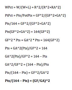
We then have the equation in an ideal form to solve for the exponent, which we will call “m”. For those of you who understand logarithms and exponents, you will know that the following formula works:

Log(Pts/(164-Pts)) = m * Log(GF/GA)

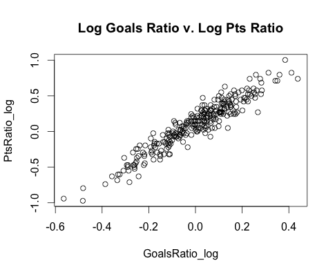
In order to find the appropriate value for m, we simply find the Log Points Ratio and Log Goals Ratio for each team in our dataset (which stretches back to 2005-2006, and from which we remove the partial 2013 season), and run a linear regression. You can see the connection between the two variables below.

The slope of this graph, and therefore the desired exponent, is 1.934, not too far away from Bill James’ original determination of 2, or from baseball’s more recent use of 1.8.

We can also try this again with only data from the past three full seasons, to see whether the result is any different as scoring continues to decrease, as is shown on the right.

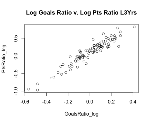
The coefficient here is 1.884, a lower number matching a lower goal scoring environment where it’s harder for teams to distinguish themselves.

The final step here is to test how will these coefficients do at predicting point differentials through linear regression. It turns out that there isn’t much difference between the two values. They both bring back R-squared values of 0.896, indicating that our formula’s expected points accounts for 89.6% of the variation in actual points for the period in question.

2. Yearly Sum of Squares

Our next method involves looping through every possible exponent value for each year in the dataset, and having our code return the one which minimizes the square of the residuals – or point differentials. By doing this, we can get a good idea of the trend in scoring, and how our exponent changes on a year-to-year basis. Here are the graphs of the values I found going through this process, first on a year by year basis, and then as a three-year rolling average.

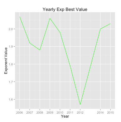
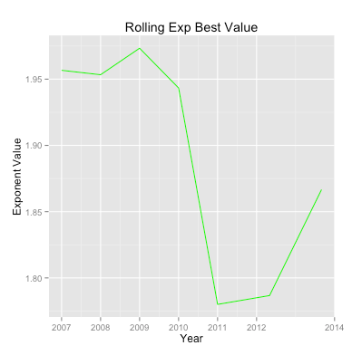
I skipped 2013 for obvious reasons, but you can see that there was a strange deviance from expectation when it came to 2012. I’ve encountered issues with 2012 data in the past, but if anybody has an explanation, feel free to share.

Once again, 2012 skews the data somewhat, but it’s clear that our initial study was accurate. The ideal exponent over the course of this data, and going forward, is likely in the range of 1.9. If you stretched the graph to 2015, that would be a value you could realistically expect to see.

3. PythagenPuck

There is one more method we can use to double check our initial estimate, and also see if we can get a superior R-squared value for our data. PythagenPuck is a method that you can read about in some detail in Ryder’s piece (which I will link to again here), and was also the subject of a piece by Travis Yost back in 2011.

 The idea behind PythagenPuck is to make your exponent variable based on the goalscoring environment of each team in the sample. So your “m” won’t be set but will rather depend on another formula completely. That formula is the following:

M = (GF/game + GA/game)^p

The idea here is that a team that sustains a higher goal-scoring environment should expect to have its expectation closer to the extremes than one which plays low scoring games. The value of p is variable, but Ryder claims that since WWII the optimal value has been about .458. I checked the results with that value and with a new value constructed with my data since the lost season. The optimal value I got was 0.48, which checks out as having a just barely higher R^2 value (0.8986 to 0.8985) than Ryder’s study stretching back farther. Ultimately, one could use either value and it wouldn’t matter all that much. PythagenPuck appears to be the best choice, and we’ll stick to Ryder’s larger sample size value for the rest of this study.